Accounting for customers’ death: a Bayesian hiearchical extension to the Pareto/NBD churn model
Published:
This post is a review of my research on customer churn patterns at Two Six Capital as a Data Scientist in 2016.
Modeling customer churn behavior is a crucial part of the bottom-up approach to forecasting business revenue based on historical customer transaction data. Retail business poses extra challenges where the customers’ “death” are not observable: customers may have churned-off permanently, which only results in no activities towards the end of the observation window. To account for the latent and heterogeneous behaviors of the retail customers, I researched and presented a Hierarchical Bayesian extension to the Pareto/NBD model that is the default model for churn at the time. In this post, I will go over the model formulation, highlight some MCMC implementation details, and present the predictive power based on simulated data.
Motivation and model formulation
The Pareto/NBD model makes the following assumptions: (i) Poisson process purchase pattern with rate $\lambda$ (ii) Exponential customer lifetime with rate $\mu$. To account for heteogeneity among the customers, the model assumes Gamma distribution for $\lambda$ and $\mu$ across population. The marginal likelihood is then Negative binomial for the purchase behavior and Pareto (of the second kind) for customer lifetime. The maximum likelihood estimates can be obtained by various optimization schemes and was used as the default by the company.
However, often times in retail business data, a customer repeat purchase behavior stops a couple of the years after entering the panel and remains dormant till the end of the observation windows. This leads to the high churn rate for initial cohort and often is not captured well by the vanilla Pareto/NBD model that models purchase and customer lifetime separately. To connect the purchase behavior and survival time on an individual level, Abe 2009 proposed the Hiearchical Bayesian extension to the Pareto/NBD model with the following formulation
Let $x_i$ be the number of transactions for customer $i$ in observation window $(0, T]$, $\tau_i$ be the latent customer survival time, and $t_{x_i}$ be the last observable transaction time.
\[x_i \sim \text{Poisson}(\lambda_i t_i), t_i = \min(\tau_i, T)\] \[\theta_i = \begin{bmatrix} \log(\lambda_i) \\ \log(\tau_i) \end{bmatrix} \sim MVN_2 \left(\boldsymbol{\mu_{0i}}, \boldsymbol{\Sigma_0}\right), \quad \boldsymbol{\theta_{0i}} = \boldsymbol{\beta}^\prime \boldsymbol{X_i}\]where $X_i$ is the covariates for customer $i$.
With this formulation, the model accounts for possible “death” of a customer before the end observation $T$ and also allows correlation between the customer lifetime and purchase rate. The latter is key for customer profiling that is often the interests to retail business analysis. Furthermore, with a Bayesian framework, meaningful inference for each individual can be derived based on posterior samples of $\mu_i$ and $\lambda_i$, e.g. a posterior distribution for mean residual life time for customer $i$ can be obtained through the posterior sample of $\mu_i$.
The posterior inference is done by first augmenting the parameter spaces with latent variable $z_i$, whether customer $i$ is alive at $T$ and $y_i$, the death time for customer $i$ if $z_i = 0$. Notice that $y_i \in [t_{x_i}, T]$. Without losing generality, I will ignore the subscript $i$ in the following derivation. The likelihood for $x, t_x \mid z, y, \mu, \lambda$ is
\[L(x, t_x \mid z = 1, y, \mu, \lambda) = P(\text{x$^{th}$ purchases at $t_x$, no purchase $(t_x, T]$| alive at T}) P(\text{alive})\\ = \frac{\lambda^x t_x^{x-1}}{(x-1)!}\exp\{-\lambda t_x\} \exp(-\lambda(T-t_x)) \exp(-\mu T)\] \[L(x, t_x \mid z = 0, y, \mu, \lambda) = P(\text{x$^{th}$ purchases at $t_x$, no purchase $(t_x, y]$ |dead at y})P(\text{dead at y}) \\ = \frac{\lambda^x t_x^{x-1}}{(x-1)!}\exp\{-\lambda t_x\} \exp(-\lambda(T-y)) \mu\exp(-\mu y)\]The joint posterior is
\begin{align} \pi(\boldsymbol{\lambda_i}, \boldsymbol{\mu}, \boldsymbol{y}, \boldsymbol{z}, \boldsymbol{\beta}|D) \propto \prod_{i = 1}^n L(x_i, t_{x_i}, T|z_i, y_i, \lambda_i, \mu_i) I_{(t_{x_i} < y_i <T)}MVN(\boldsymbol{\theta_i}|\boldsymbol{\mu_{0i}}, \boldsymbol{\Sigma}) \pi(z_i)\pi(\boldsymbol{\beta}, \Sigma)
\end{align}
Posterior inference highlight
Update $y_i$
Notice that the full conditional for $y_i$ when $z_i = 0$ is a truncated exponential with rate $\mu_i + \lambda_i$ and truncation such that $t_{x_i} < y_i < T$. I used slice sampling technique to update the $y_i$.
Update $z_i$
We can integrate $y$ out to obtain the likelihood for $x, t_x \mid z = 0, \mu, \lambda$
\[L(x, t_x \mid z = 0, \mu, \lambda) = \frac{\lambda^x t_x^{x-1}}{(x-1)!}\exp\{-\lambda t_x\}\int_{t_x}^T \exp(-\lambda(T-y)) \mu\exp(-\mu y) dy \\ = \frac{\lambda^x t_x^{x-1}}{(x-1)!}\exp\{-\lambda t_x\}\frac{\mu}{ \mu + \lambda} \exp(-(\lambda + \mu)(T-y))\]Assume Bernoulli prior for $z$, $\pi(z = 0) = \pi(z = 1) = 0.5 $, the full conditional for $z$ is
\[\pi(z = 1) = \frac{1}{1 + \frac{\mu}{\mu+\lambda}}\exp\{(\mu + \lambda)(T-t_x) - 1\}\]Then $z_i$ is updated by sampling from the updated Bernoulli with $p = \pi(z = 1)$.
The full conditional for $\theta_i$ does not have closed-form. A standard Metropolis update was implemented. The coefficients are updated through standard MVN-MVN Inverse Wishart updates.
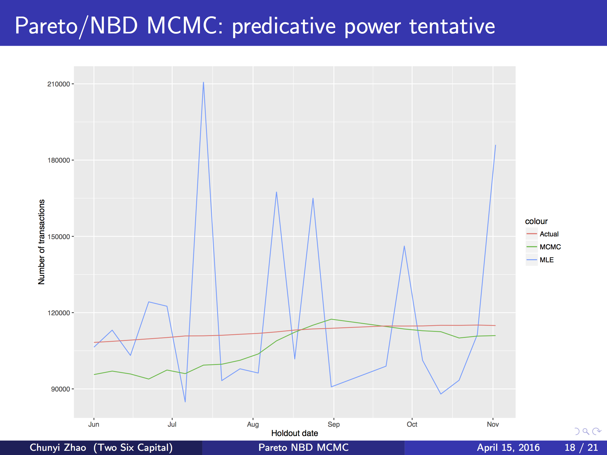
Simulation study and model comparison
I implemented the HB extension to the Pareto/NBD model and applied it to simulated data where customers can churn-off permenently. The forecasting result using the HB extension is drastically superior than that based on vanilla Pareto/NBD.
In conclusion, the HB extension can provide more meaningful inference and better forecasting performance. However, the computation cost increases significantly if the total number of customers is large.
The original talk is linked here
The git repo is linked here