BNP prior series: From Gaussian Process to Gaussian Markov Random Field: many GP related models applied to Albeto data
Published:
In this post, I will review class projects in STAT 245 Spatial Statistics. The main models include stationary Gaussian Processes Bayesian inference, Predictive Gaussian Process, and finally Gaussian Markov Random Field. The goal is to highlight model properties, implementation details, and present some real data analysis with these three models applied to the Albedo satellite data in North America.
Data
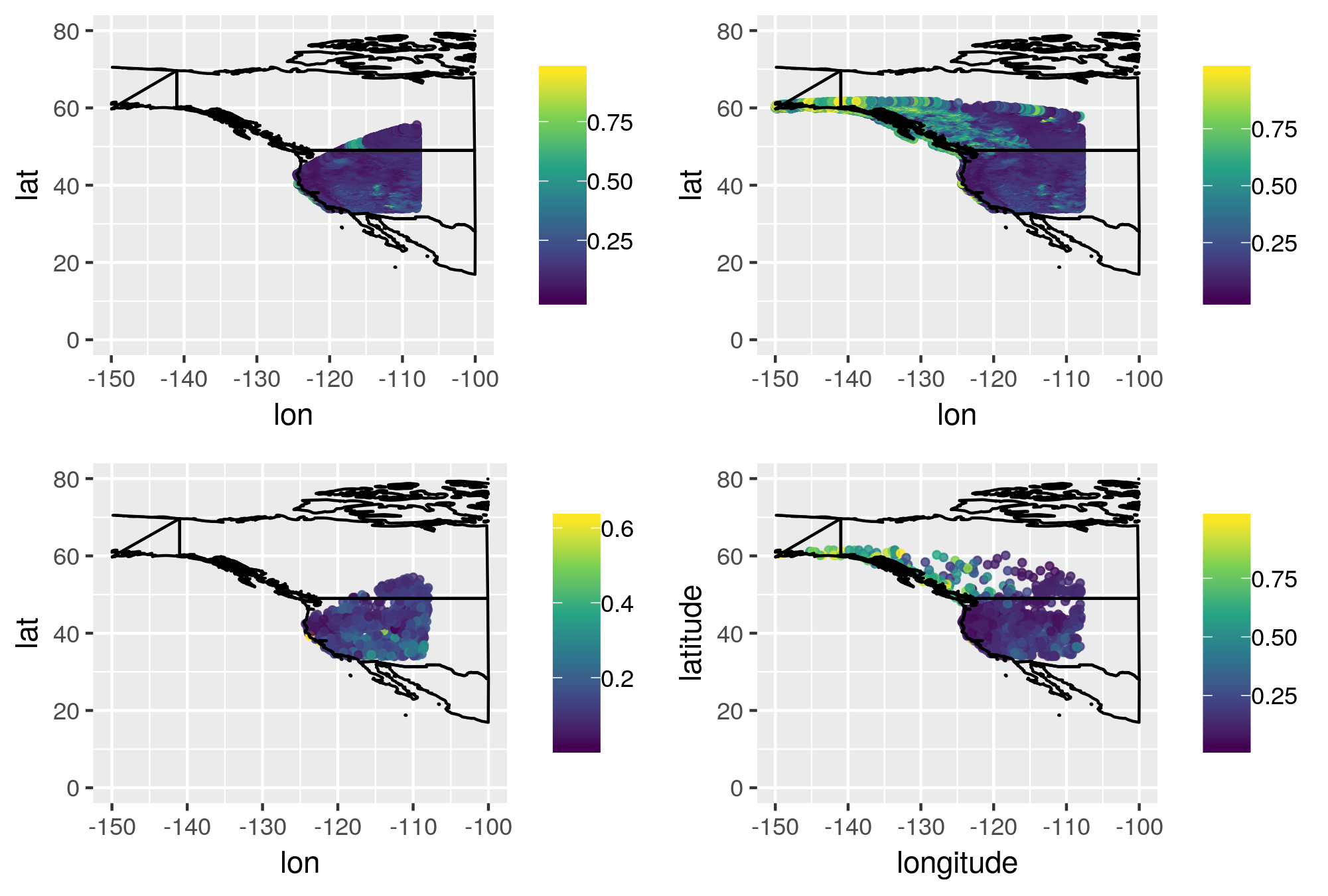
Albedo is the proportion of light or radiation reflected by surface. We are interested in Albedo over land, since its variation over the ocean is small. To control project scope, the training data was obtained by sampling 500 locations each within the the block with lon $[-126, -108]$ and lat $[34, 62]$ among 0.19 million points for the two Satellites A and B. Locations within the ocean are intentionally removed.
- Raw and sampled data from two Satellites: left col: A, right col: B, top row: raw, bottom row: sampled
Modeling methods
In this section, I will review three models implemented in the class projects to model Albedo with the data described above: 1) a hierarchical Bayesian GP with Matern covariance function applied to two Satellite training data separately, 2) a predictive Gaussian Process with Matern covariance function applied to two Satellite training data separately, 3) a Kernel convolution approach that models the two satellite data together, accounting for the common mean effect and difference effect between the two. The latter two approaches are both low-rank approximation of Gaussian process that are computationally more efficient but not stationary. The last approach models the replicates of the same measure jointly in the same model.
1. Guassian process with Matern correlation functions
Let the logit transformed Albedo or weighted Albedo be $Y(s)$, the design matrix $D(s)$ is a $500 \times 3$ matrix where the columns are vector of ones, longitude and latitude. Assume nugget effect, let $\gamma^2 = \frac{\tau^2}{\sigma^2}$, where $\tau^2$ is the nugget and $\sigma^2$ is the partial sill. A Bayesian model is then formulated in the following hierarchical way:
\(Y(s) \sim MVN_n(X(s)\beta, \tau^2(I_n + R(\phi, \nu)/\gamma^2))\) Let $V = I_n + R(\phi, \nu)/ \gamma^2$.
Place improper prior on $\beta$ and inverse-gamma prior on $\tau^2$ \(\pi(\beta, \tau^2) \propto IG(\tau^2|2, 1)\)
The marginal likelihood of $\phi, \gamma^2, \nu$ is obtained by integrating out $\beta, \tau^2$:
\[L(\phi, \gamma^2, \nu) \propto |V|^{-\frac{1}{2}}|D'V^{-1}D|^{-\frac{1}{2}}S(\phi, \gamma^2, \nu)^{-\frac{n-k-2}{2}}\]where $S(\phi, \gamma^2, \nu)$ is the weighted LSE residual, and $k$ is the number of columns of the design matrix.
A uniform prior is placed on the nugget/sill ratio $(1 + 1/\gamma^2)^{-1}$, since this ratio is truly between 0 and 1 at all time. A uniform prior is placed on range parameter $\phi$. Finally as the smoothness parameter $\nu$ typically takes values $1/2, 3/2, 5/2$, at which the computation of covariance matrix is fast. To make the model fully Bayesian, I considered two types of prior on $\nu$: 1)place a uniform prior on $\nu$ and sample $\nu$ in a joint Metropolis-Hastings step along with $\phi$ and $\gamma^2$. 2) create a latent variable z for $\nu$ such that $\nu = 1/2$ if $z \in (0, 1]$, $\nu = 3/2$ if $z \in (1, 2]$ and $\nu = 5/2$ if $z \in (2, 3]$, and jointly update z in a MH step with $\phi$ and $\gamma^2$.However, these two approaches lead to bad mixing. So I eventually fixed $\nu$ at its marginal MAP estimates, and sampled $\phi, \gamma^2$ over a discrete grid. The grid search approach is 10-20 times computationally more efficient than the other two approach. I will describe the details of this approach in the next section.
1.1 Implementation details
grid search over $\phi$, $\gamma^2$, fix $\nu$ at MAP
A MAP estimation is performed based on the marginal joint posterior distribution for $\phi, \gamma^2, \nu$. The marginal posterior for $\phi, \gamma^2, \nu$ based on the prior choices discussed before is
\[p(\phi, \gamma^2, \nu \mid y) \propto \mid V\mid^{-\frac{1}{2}}|D'V^{-1}D|^{-\frac{1}{2}}(S(\phi, \gamma^2, \nu)+1)^{-\frac{n-k}{2}-2}\]Fix $\nu$ at $\tilde{\nu}$, create a grid for $\phi$ and $\gamma^2$ that includes their MAP estimates.
The marginal posteriors for all the choices over the grid are then computed, the sufficient statistics $\hat{\beta} = (D’V^{-1}D)^{-1}D’V^{-1}y$ and $S(\phi, \gamma^2, \nu) = \mid \mid y-D\hat{\beta}\mid \mid ^2$ is calculated along the way and stored in dictionary. For each iteration of MCMC, first sample values for $\phi, \gamma^2$ using weights as marginal posteriors, and sample $\beta$ and $\tau^2$ with Gibbs update using pre-computed sufficient statistics for the given choice of $\phi, \gamma^2$. The algorithm is 10-20 times faster than the other two approach and performs fairly stably.
2. the Predictive Gaussian Process
From the original GP model \(y_i = f(x_i) + \epsilon_i\)
\[f(x) \sim GP(\mu, \tau^2 exp(\phi d))\]Let $x_1^\ast, \cdots, x_s^\ast$ be a set of knots.
Define
\(f^\ast = [f(x_1^\ast), \cdots, f(x_s^\ast)]\) \(cov(f(x_i), f^\ast) = [\rho(x_i, x_1^\ast \mid\theta), \cdots, \rho(x_i, x_s^\ast \mid\theta)]\) where $\rho$ is the covariance function defined through parameter $\theta$.
\[Var(f^\ast)_{i, j} = (\rho(x_i^\ast, x_j^\ast \mid\theta)) = C^{\ast -1}\]Using the conditional distribution of MVN, we have \(y_i = \mu + cov(f(x_i), f^\ast)^T Var(f^\ast)^{-1}f^\ast + \epsilon_i\)
In matrix form this is, \(y = \mu + [c(x_1), \cdots c(x_n)]C^{\ast-1}f^\ast + \epsilon\)
\[C^{\ast-1} = Var(f^\ast)\]We define $K$ matrix in the kernel convolution by $K = [c(x_1)^\prime; \cdots; c(x_s)^\prime]C^{\ast -1}$. Where $c(x_1) = [\rho(x_1, x_1^{\ast}), \cdots, \rho(x_1, x_s^{\ast})]$.
So equivalently \(y = \mu + Kf^\ast + \epsilon\)
Posterior inference of this model is done using R package spBayes.
2.1 Predictive GP model properties
The advantage of using Predictive DP is not only that it reduces computation as a Low-Ranked method, it also has reduced variability compared to the full GP model.
The full model,
\(y_i = \mu + f(x_i) + \epsilon_i\)
The predictive process \(y_i = \mu + cov(f(x_i), f^\ast)var(f^\ast)^{-1}f^\ast + \epsilon\)
\[cov(f(x_i), f^\ast)var(f^\ast)^{-1}f^\ast = E[f(x_i)\mid f^\ast]\]Thus the predictive process is
\[y_i = \mu + E[f(x_i)\mid f^\ast] + \tilde{\epsilon_i}\]When working of the full model, the variability of the full model \(Var(f(x_i)) + \sigma^2\)
$\sigma^2$ is the noise
The variability of the predictive process is \(Var(E[f(x_i)\mid f^\ast]) + \tilde{\sigma^2}\)
The difference in variability of regression function = $var(f(x_i))- var(E[f(x_i)\mid f^\ast]) = E[Var(f(x_i)\mid f^\ast)]$
We can therefore strictly reduce the variance of our estimator.
3. GMRF
The spatial effect is modeled through a process convolution of spherical Bezier kernel and a GMRF prior on the coefficients. The transformed data $Y_1(s^{(1)})$ is a vector of $n_1$ observations at locations $s^{(1)}$ from the first data source, i.e Satellite A; $Y_2(s^{(2)})$ is the vector of $n_2$ observations at locations $s^{(2)}$ from the second data source, i.e. Satellite B. $X_1$ and $X_2$ are $n_1 \times k_1$, $n_2 \times k_2$ covariates matrices for GOES 135 and GOES 075 respectively. Let $\boldsymbol{\beta_1}$ and $\boldsymbol{\beta_2}$ be $k_1 \times 1$, $k_2 \times 1$ coefficient vectors for GOES 135 and GOES 075. The model is formulated in the following way:
\[\begin{bmatrix} Y_1(s^{(1)}) \\ \ Y_2(s^{(2)}) \end{bmatrix} = \begin{bmatrix} X_1 & 0 \\ 0 & X2 \end{bmatrix} \begin{bmatrix} \boldsymbol{\beta_1}\\ \boldsymbol{\beta_2} \end{bmatrix} + \begin{bmatrix} K_\mu^{(1)} & 0 \\ K_\mu^{(2)} & K_\delta^{(2)} \end{bmatrix}\begin{bmatrix} \boldsymbol{Z_\mu}\\ \boldsymbol{Z_\delta} \end{bmatrix} + \begin{bmatrix} \boldsymbol{\epsilon_1}\\ \boldsymbol{\epsilon_2} \end{bmatrix}\] \[\begin{bmatrix} \boldsymbol{\epsilon_1}\\ \boldsymbol{\epsilon_2} \end{bmatrix} \sim MVN_{n_1 + n_2}(\boldsymbol{0}, I_{n_1 + n_2} \tau^2)\]where $K_\mu^{(1)}$ is the $n_1 \times p$ kernel matrix for GOES 135 mean effect, $K_\mu^{(2)}$ is the $n_2 \times p$ kernel matrix for GOES 075 mean effect, $K_\delta^{(2)}$ is the $n_2 \times p$ kernel matrix for GOES 075. All three kernels are defined with the observation location for each satellite and a set of common knots $[u_1, \cdots, u_p]$. The box The spherical Bezier kernel with range $r$ and power $\nu$ is defined as
\[b(s_i, u_j) = (1- (\frac{\mid\mid s_i-u_j \mid \mid}{r})^2)^{\nu} I_{[\mid \mid s_i-u_j\mid \mid < r]}\]where $\mid \mid s_i-u_j\mid \mid$ is the distance between observation at location $s_i$ and knot at location $u_j$. In the following implementation, I use great-circle distance to construct the Bezier kernel. $\nu$ is fixed at 1.0 for 3 kernel matrices. The range parameter differs for the mean process and difference process as $r_\mu$ and $r_\delta$ respectively. Thus $K_\mu^{(1)}$ and $K_\mu^{(2)}$ are calculated using $r_\mu$ and $K_\delta^{(2)}$ is calculated using $r_\delta$.
To complete the model, GMRF prior is placed on $Z_1$ and $Z_2$ with the same set of knots for both process. The common component in the precision matrix, i.e. adjacency matrix $W$ is defined as
\[W_{ij} = n_i I_{[i = j]} - I_{[i \sim j, i \neq j]}\]where $n_i$ is the number of neighbors knots $i$ has. $i \sim j$ means knot $i$ and knot $j$ are adjacent to each other in the first order, i.e. j is either directly above, below, or next to i from left or right. On a regular grid, the inner knots always have 4 adjacent neighbors; the edge knots have 3 neighbors and the corner knots have only 2.
Finally GMRF prior is placed on $Z_\mu$ and $Z_\delta$ with precision parameters $\lambda_\mu$ and $\lambda_\delta$
\[Z_\mu \sim GMRF(\lambda_\mu W) \quad Z_\delta \sim GMRF(\lambda_\delta W)\]The following priors are placed on $\tau^2$, $\lambda_1$ and $\lambda_2$ \(\tau^2 \sim IG(2.0, 1.0) \quad \lambda_\mu \sim Ga(2.0, 1.0) \quad \lambda_\delta \sim Ga(2.0, 1.0)\)
3.1 Full conditionals
The simulation-based inference employs a Gibbs sampler to obtain samples of parameters $[\beta_1, \beta_2, Z_\mu, Z_\delta, \lambda_\mu, \lambda_\delta, \tau^2]$ from the following full conditionals
\[\beta_1|- \sim MVN_{k_1}((X_1'X_1)^{-1}X_1'(Y_1-K_\mu^{(1)}Z_\mu), (X_1'X_1)^{-1}\tau^2)\] \[\beta_2|- \sim MVN_{k_2}((X_2'X_2)^{-1}X_2'(Y_2-K_\mu^{(2)}Z_\mu - K_\delta^{(2)}Z_\delta), (X_2'X_2)^{-1}\tau^2)\] \[V_\mu =((K_\mu^{(1)'} K_\mu^{(1)} + K_\mu^{(2)'} K_\mu^{(2)})/\tau^2 + \lambda_\mu W)^{-1}\] \[A = (Y_1 - X_1\beta_1)'K_\mu^{(1)}/\tau^2 +(Y_2 - X_2\beta_2 - K_\delta^{(2)}Z_\delta)'K_\mu^{(2)}/\tau^2\] \[Z_\mu| - \sim MVN_{p}(V_\mu A', V_\mu)\] \[V_\delta=((K_\mu^{(2)'}K_\mu^{(2)})/\tau^2 + \lambda_\delta Z_\delta)^{-1}\] \[Z_\delta \mid - \sim MVN_p(V_\delta K_\delta^{(2)'}(Y_2 - X_2 \beta_2 - K_\mu^{(2)}Z_\mu), V_\delta)\] \[\lambda_\mu| - Ga(a_\lambda + r(W), b_\lambda + Z_\mu'W Z_\mu/2) \quad \lambda_\delta| - Ga(a_\lambda + r(W), b_\lambda + Z_\delta'W Z_\delta/2)\]where $r(W)$ is the rank for W.
\(\tau^2|- \sim IG(2 + (n_1+n_2)/2, SSE_1/2 + SSE_2/2 + 1)\) where $SSE$ is the sum of square residuals for $Y_1$ and $Y_2$.
Kriging results
Here are some selected kriging results based on the latter two approaches
- Kriging result for Satellite A using Predictive GP
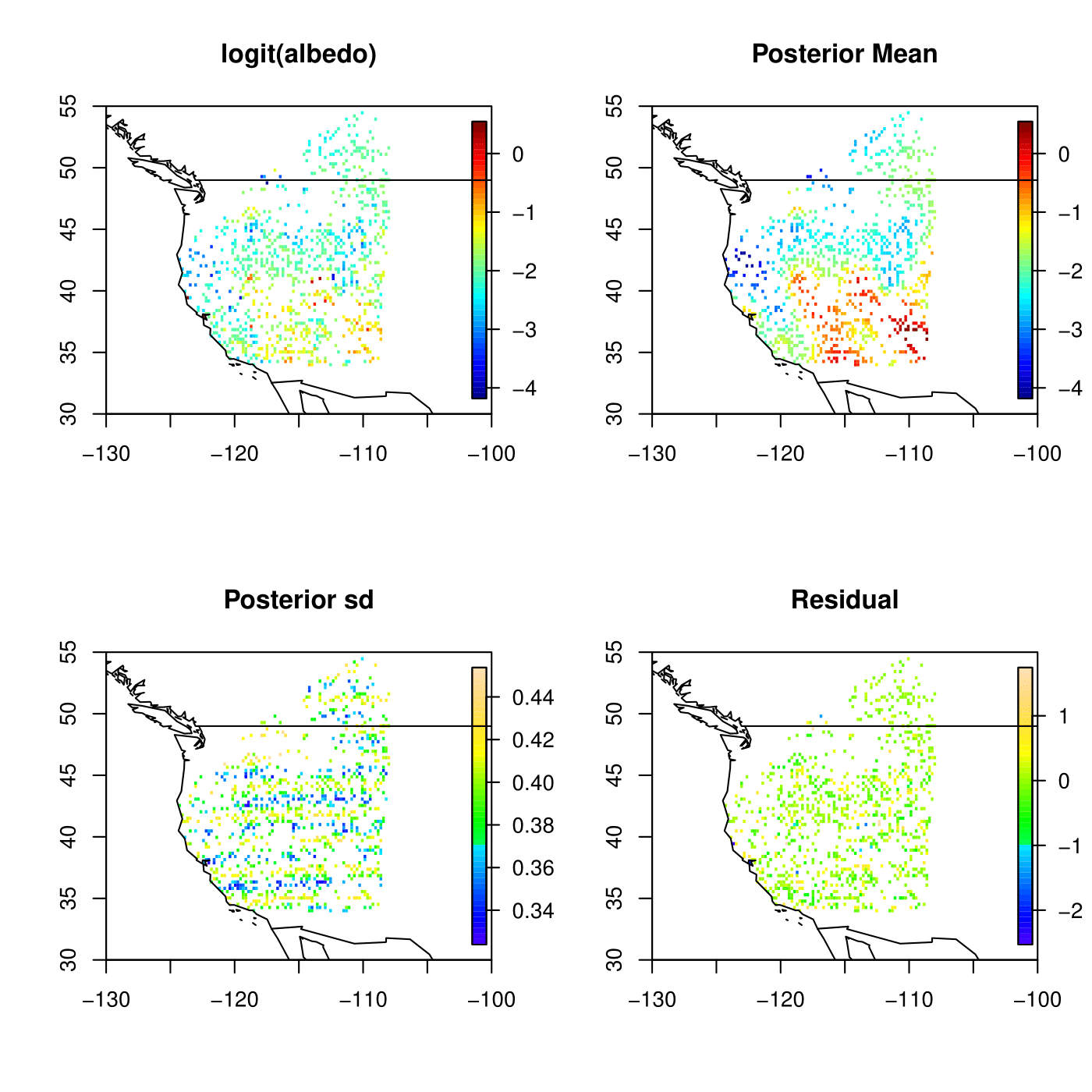
Kriging result for Satellite B using Predictive GP
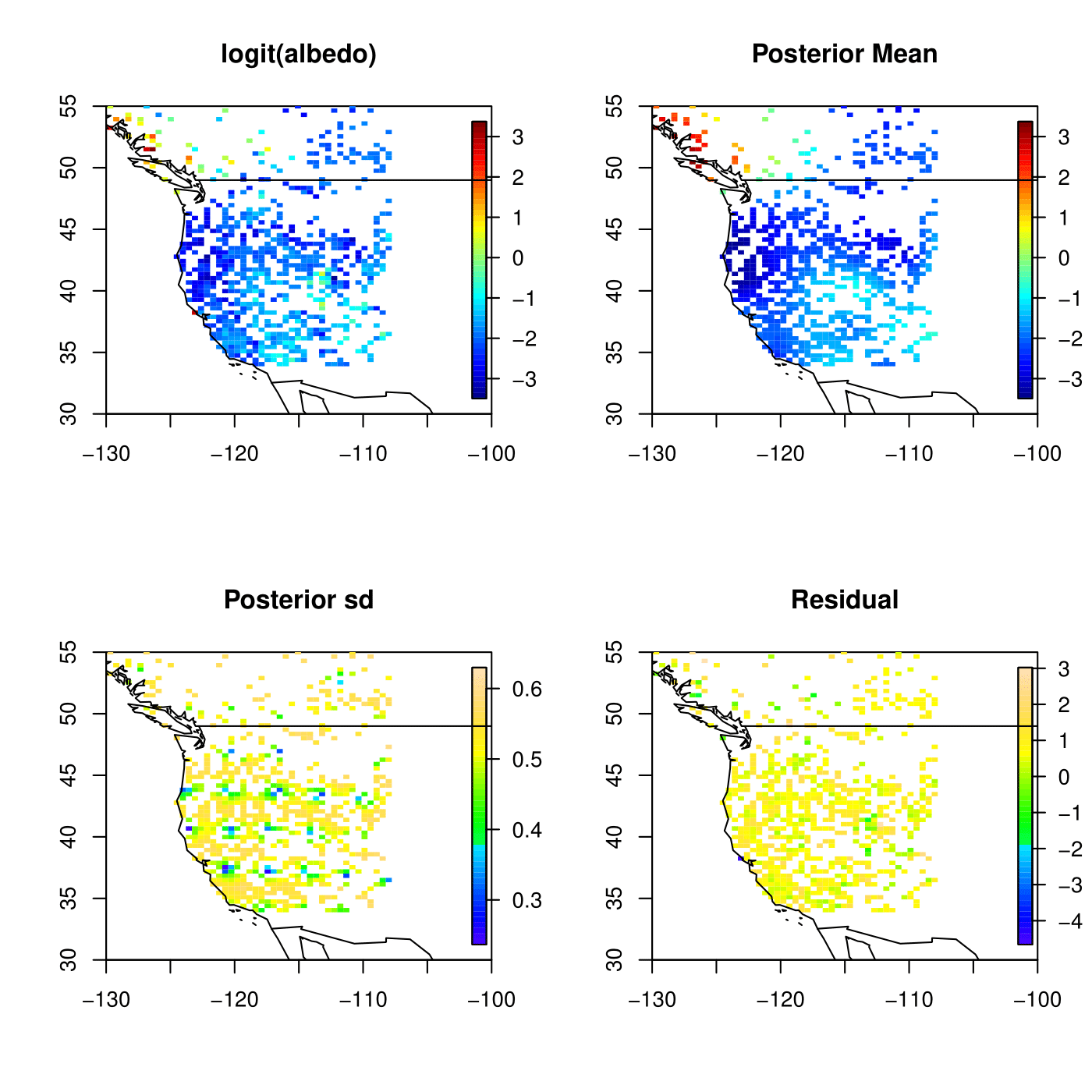
Kriging result for Satellite A using GMRF

Kriging result for Satellite B using GMRF
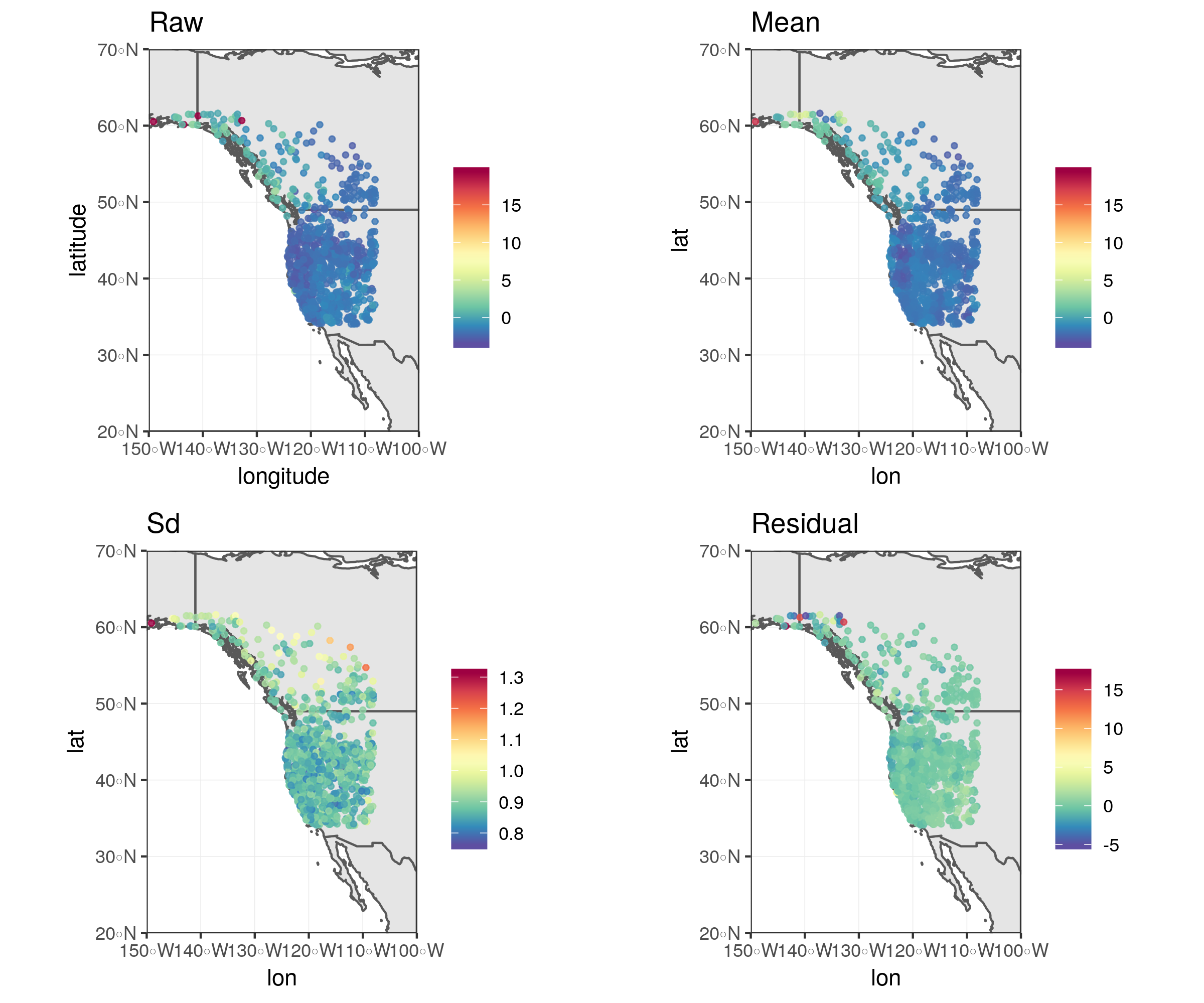
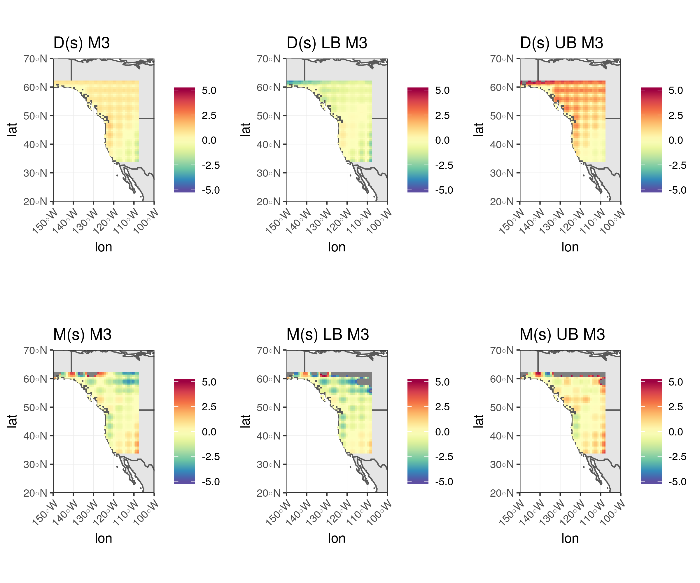
Inference for latent mean and difference processes using GMRF